There are a lot of different ways to analyze cost calculations. Give below are more details for some of the different analyses.
Use this function for analyzing cost build-up over time. The product structure and the lead time, along with the costs associated with the parts and its components, make up the costs shown in the graph. This can be used to improve business and restructure the Bill of Material (BOM) so that large expenses are pushed as forward as possible. Lead time cost can be calculated only for manufactured parts.
Use this function to analyze the break-even sales point or volume depending on a part's costs. This can be useful when setting the sales price and estimating the sales volume. Cost-Volume-Profit Analysis performance at specific levels such as Part Number, Structure Alternative, Routing Alternative, Site and Cost Set is available.
There are three different analyses: Break-Even Analysis, Sensitivity Analysis and Optimal Price Calculation. You can also calculate the part's Estimated Elasticity and use the elasticity value in the Cost-Volume-Profit Analysis.
This analysis uses the Delphi methodology to determine the price elasticity
of the part.
The formula to calculate estimate price elasticity is as follows.
E = P1 - P2 x V1
P1 V1 - V2
where E = Estimated Elasticity
P1 = Price 1
P2 = Price 2
V1 = Volume 1
V2 = Volume 2
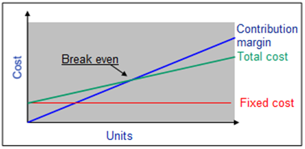
The break-even analysis can be done in three different ways:

Figure 1 - Break Even Analysis
The cost base used in the following examples is variable cost.
If a sales price and fixed cost are entered, this tool calculates the break-even
volume as follows:
Fixed Cost/(Unit Price - Variable Cost) = B/E Volume
If a break-even volume and fixed cost are entered, this tool calculates the break-even price as follows:
Fixed Cost + (Variable Cost * Unit Volume)/Unit Volume = B/E Unit Price
If an ROS and a fixed cost are entered, this tool calculates the break-even price and volume as follows:
Variable Cost/[1 - (ROS/100)] = B/E Unit Price
Fixed Cost/[B/E Unit Price (ROS) - Variable Cost] = B/E Volume
Entering return on investment (ROI) is independent of the analysis type.
Price or ROI as analysis type calculates ROI volume as follows:
(Fixed Cost * (ROI/100) + Fixed Cost)/(Price -Variable Cost)
Volume as analysis type calculates ROI price as follows:
((Fixed Cost * (ROI/100) + Fixed Cost)/Volume) + Variable Cost
Entering Safety Margin
Safety volume is always calculated as follows:
Break-Even Volume/[1 - (Safety Margin/100)]
Break-Even volume is calculated as follows:
Safety Volume * [1 - (Safety Margin/100)]
If volume is selected as the analysis type, the volume entered is regarded as safety volume.
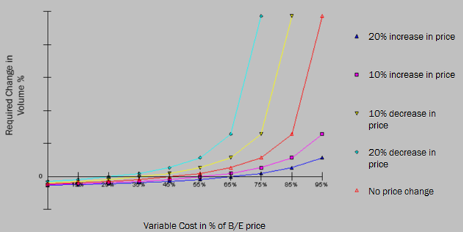
Use this function to see how price changes affect the volume. A break-even (B/E) analysis must be performed. It shows how the variable cost of the B/E price as a percentage requires changes in the percentage of volume, at a price increase or decrease of 10% or 20%.

Figure 2 - Sensitivity Analysis
Use this function to see the result of a break-even analysis in graph form for both price and volume.
There are difference ways to analyze variances between two different cost sets for a part, in the Part Cost Variance window it shows the variances on a high level and in the Part Cost Variance window it shows the variance for each included cost bucket for the part in the calculations.
In the Part Cost Variance window you can compare and analyze differences between cost sets:
This analysis can be useful to calculate new costs for the next
period and it will be easy to see the differences between old and new costs.
In
the Part Cost Variance
window you have three options that you can select to
specify the variances for the part and the Cost Set that you have select to
compare between:
Show All Cost Buckets Indicator - this option is selected by default
Set Minimum Variance Factor - the buckets shown are those that differ in total or level cost more than the specified minimum variance. The minimum variance is calculated as the ((Left Value – Right Value)/Left Value) > Minimum variance
Set Maximum Variance Factor - the buckets shown are those that differ in total
or level cost more than the specified maximum variance. The maximum variance is
calculated as the ((Left Value – Right Value)/Left Value) < Maximum Variance
This analyze can be useful to determine the buckets in which differences exist
in total costs for a part in different cost sets.
Use this function to see the cost information for a selected part. You can view cost set information, cost bucket information and cost template information related to the part. To use this the costs must have been calculated for the part.
In the Part Cost History Graph window you can follow how a part's cost have developed over time. The graph shows both the accumulated cost as well as level cost. You can select for period and type of period you will see the graph.
Use the Component Cost Build-Up Graph window to see how components contribute to the total accumulated cost for the actual part. The component are sorted by how much they contribute to the total accumulated cost, with the most expensive component first.
Use this functionality to analyze the unit cost per lot size, to use this total cost for the part must be calculated and a lot size must be defined. The graph shows the effects of the set up costs, depending on the Lot Size you calculate on. This function does not consider carrying costs.
Use this function to analyze part routing cost or to simulate cost for a routing alternate. You can analyze routing cost for cost calculation generated:
If you simulate cost, only one record will be saved for each part number, cost
set and alternate/revision, so if you simulate more than once with different lot
sizes only the last simulation will be saved.
There are two tabs with pie chart; one for cost per operation and one for cost
per cost type, those gives you a quick answer over the distribution of costs for
the routing.
Use this function to analyze cost of a specific configuration for a configured part. To do this the cost calculation must have performed for the configured part you want to analyze.
Use this function to evaluate the reusability of components within product structures. You can do this for both manufactured and purchased part costs.
There are two parameters that have to be set:
The product family and product code must be set and calculated within the product structure. The parameters are set in IFS/Inventory Part, and calculated using the Update Product Family and Product Code dialog box. Product family will give an identity to a family group at a high level. The product code gives an identity on a lower level. The next level is identity by part number.
The cost calculation at all levels:
Cost calculation gives information about manufacturing cost and purchase cost
both in cumulated cost, as well as level cost. Parts at the same site will be
measured for commonality/uniqueness when it comes to manufacturing cost,
purchase cost, and number of parts, concerning both product family and product
code identity.
When the the product family and product code is updated, and it comes across a component part that belongs to more than one product structure, the following happens:
If, for example, the product family values of the different parent parts are the same, then nothing happens (the product family of the component part is considered unique, and retains its value, e.g., men's bikes). If, on the other hand, the product family values of the different parent parts are not the same, the product family of the component part is considered common, and is given the value * (asterisk). A person responsible for system changes can optionally have some other value representing common components, but the system default is always asterisk.
The exact same rules also apply to product code.
The calculation excludes master schedule phantom parts, i.e., parts with planning method O or T.
Use this function to evaluate the Cost/Importance relation for a part structure. The relative importance is produced by assigning feature importance to each components within the structure.
Cost value analysis helps you to determine whether there are any customer
requirements related to any function of the product. Functions are related to
parts within the part structure. The knowledge of customer requirements makes it
easier to conduct product rationalization.